Extracting and visualizing `verywise` results

Serena Defina

2026-06-09

verywise output

Check out the output directory. You should see something like this

[TODO: add image]

Extracting mean/median cluster values

Sometimes, you may want to extract the mean or the median value of a specific cluster from your results, for example to use this in further analysis. You can do this in verywise using the significant_cluster_stats() function.

Note: ideally, you should run your analyses with save_ss = TRUE or save_ss = "path/to/ss", or you have called build_supersubject() in your pipeline, for this to sun smoothly.

# Extract mean from significant clusters
df <- significant_cluster_stats(stat = "mean", # or "median"
                                ss_dir = "path/to/ss_directory", 
                                res_dir = "path/to/results", 
                                term = "age", # term of interest 
                                measure = "thickness", 
                                hemi = "lh")

Visualizing results

verywiseWIZard: interactive visualization app

To inspect and plot your results, you can use our interactive web application, verywiseWIZard. You can run this locally or try it out here.

Note: if you are using the online version of the WIZard, with results hosted on GitHub, you may want to look into the move_result_files() helper function, to organize your results in a way that is safe (i.e., does not expose individual level data) and quick.

verywise plotting functions

Plots can also be generated using verywise directly. You can use these functions in R, but they are Python wrappers, so they will require the reticulate package installed.

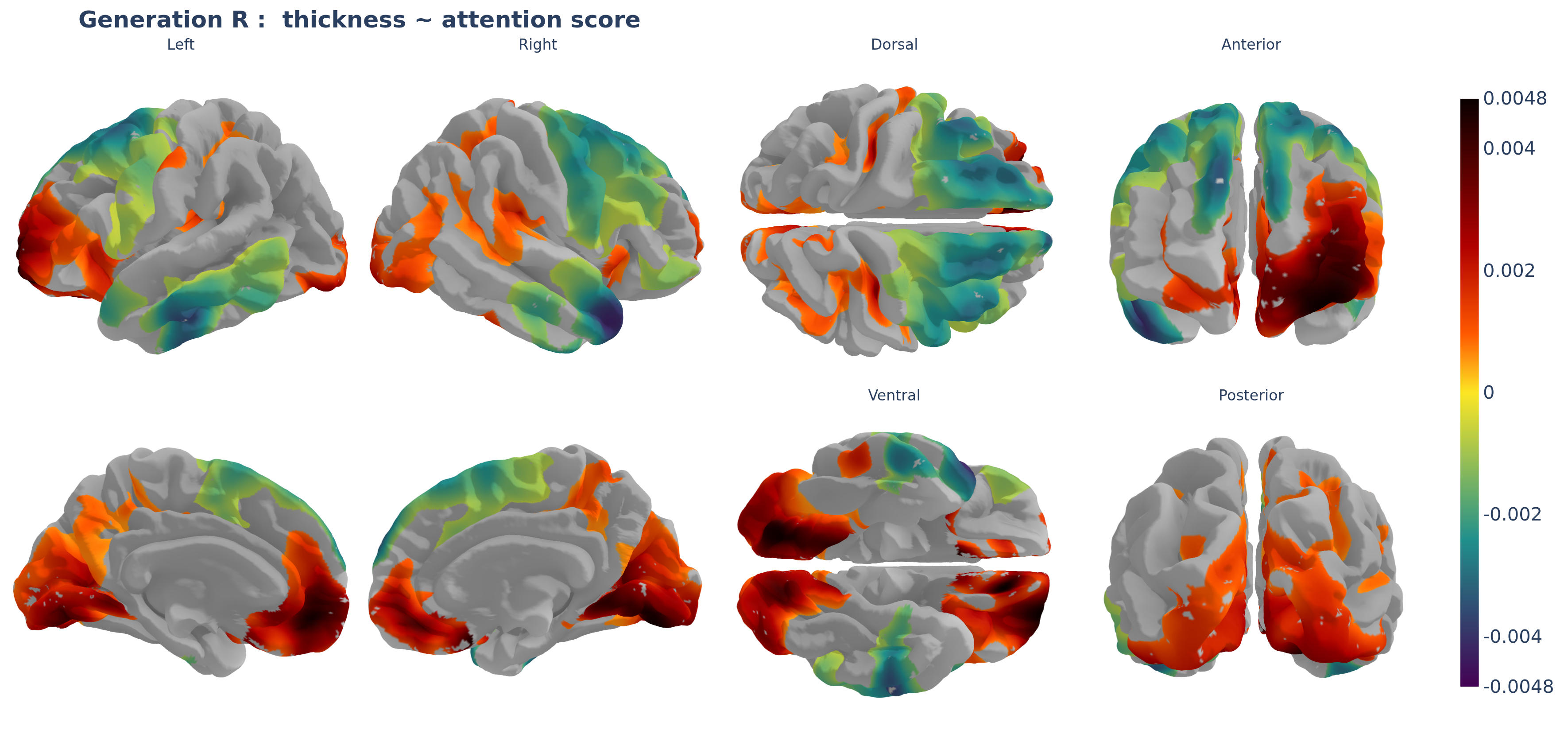
You can plot (thresholded) estimate maps like so:

plot_vw_map(
  res_dir = "/path/to/output",
  term = "age",
  measure = 'area', 
  hemi = "both", # (default) or "lh", "rh" for single hemisphere
  surface = "pial", # or "inflated"
  threshold = 'fdr<0.05',
  to_file = NULL, # interactive visualization or static output
  # optional argument 
  fs_template = "fsaverage",
  fs_home = "/path/to/FREESURFER_HOME", # quicker: use local maps 
  # outline_rois = c("entorhinal", "precuneus") # TODO: not yet available
)

The threshold argument can be one of:

• "cws" for cluster-wise significant (the default) - provided that such clusters were estimated at the analysis stage
• "fdr<0.05" for other multiple testing corrected thresholds (such as FDR) - provided that these were estimated at the analysis stage
• a numeric value e.g. 0.001 which is interpreted as a beta value threshold,

When to_file= NULL verywise will try to open an 3D interactive visualization of the brain map in the Viewer window (e.g. in RStudio) or the default browser. This can be saved as an HTML file, but often you may prefer a “static” PNG image were the all the brain is visible. This can be obtained by setting to_file = path/to/figure.png or similar output file path. The figures will then look similar to this:

Another useful function is plot_vw_diff() and plot_vw_surf()

On an HCP cluster

If you want to make plots directly on an HPC cluster (e.g. Snellius) you will need to have some version of chrome installed (kaleido one works) and set up an Xvfb process before starting R (e.g. in your job script or in the shell before launching R):

For example, on Snellius, I do:

module load 2025
module load Xvfb/21.1.18-GCCcore-14.2.0

Xvfb :99 -screen 0 1280x1024x24 &
export DISPLAY=:99
sleep 1  # give Xvfb time to start

Troubleshooting:

# check for existing Xvfb processed running on this node 
ps aux | grep -i "Xvfb.*:99"

Next article: Run vertex-wise federated / meta- analyses